In industrial process control, environmental monitoring, and laboratory analysis, conductivity measurement is a critical physicochemical parameter for quantifying ionic concentration in aqueous solutions—governed by international standards (e.g., IEC 60746-3:2018, ASTM D1125-23). Traditional electrode-based conductivity sensors (two-electrode/four-electrode designs) face inherent limitations in harsh environments: electrode fouling from biofilm or sediment, corrosion from strong acids/bases, and contamination risks in high-purity applications. Toroidal conductivity sensors (also called inductive or electrodeless conductivity sensors) address these challenges by leveraging electromagnetic induction for contactless measurement, making them indispensable for industrial processes requiring long-term reliability, low maintenance, and wide conductivity range coverage.  

 

This article delves into the technical principles, structural design, performance advantages, industrial applications, and selection criteria of toroidal conductivity sensors—providing a technical framework for process engineers, laboratory technicians, and facility managers seeking to optimize conductivity monitoring in critical systems.  

 

1.1 Definition of Conductivity  

Conductivity (σ, measured in Siemens per meter, S/m) quantifies a solution’s ability to conduct electric current, proportional to the concentration, mobility, and valence of dissolved ions (e.g., Na⁺, Cl⁻, Ca²⁺). For industrial applications, conductivity is often reported as specific conductivity (corrected to 25°C via temperature compensation) to eliminate environmental variability. Key unit conversions:  

- 1 S/m = 10 mS/cm = 10,000 μS/cm  

- Ultra-pure water: ~0.055 μS/cm (25°C); seawater: ~5 S/m (25°C); industrial brines: >10 S/m.  

 

1.2 Classification of Conductivity Sensors  

Conductivity sensors are categorized by measurement principle, each tailored to specific applications:  

 

| Sensor Type | Measurement Principle | Key Specs (Typical) | Limitations | Primary Applications |  

|-------------|-----------------------|---------------------|-------------|----------------------|  

| Two-Electrode Sensors | Direct current flow between metal electrodes (e.g., platinum, graphite) | Range: 0.1 μS/cm–20 mS/cm; Accuracy: ±1% FS | Electrode fouling/corrosion; limited to low-to-medium conductivity | Laboratory analysis, drinking water monitoring |  

| Four-Electrode Sensors | Current applied via outer electrodes; voltage measured via inner electrodes (reduces polarization) | Range: 1 μS/cm–1 S/m; Accuracy: ±0.5% FS | Susceptible to fouling in high-turbidity solutions | Municipal wastewater, moderate industrial streams |  

| Toroidal (Inductive) Sensors | Electromagnetic induction between two toroidal coils (no direct contact) | Range: 0.01 μS/cm–20 S/m; Accuracy: ±0.5% FS | Higher power consumption than electrode-based | Harsh industrial environments, high-purity water, high-salinity brines |  

| Ultra-Low Conductivity (ULC) Sensors | Specialized toroidal/four-electrode design for trace ionic measurement | Range: 0.01–10 μS/cm; Accuracy: ±0.1 μS/cm | Sensitive to environmental interference | Pharmaceutical water (USP <1 μS/cm), semiconductor manufacturing |  

 

Toroidal sensors stand out for their contactless operation, making them the preferred choice for aggressive, fouling-prone, or high-purity matrices.  

 

Toroidal conductivity sensors operate on the principle of electromagnetic induction (Faraday’s Law of Electromagnetic Induction), eliminating the need for direct electrode-solution contact. Below is a detailed breakdown of their structure and operational workflow:  

 

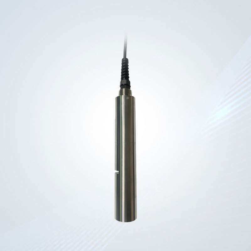
2.1 Structural Design  

A toroidal sensor consists of two concentric, toroid-shaped wire coils (typically copper or silver-plated copper) encapsulated in a chemically resistant polymer housing (e.g., PPS, PVDF, Teflon®). Key components:  

- Driving Coil (Transmitter Coil): Connected to a high-frequency alternating current (AC) source (1–10 MHz, frequency optimized for conductivity range). Generates a time-varying magnetic field (B) perpendicular to the coil plane.  

- Receiving Coil (Detector Coil): Positioned concentrically around the driving coil. Induces a voltage (V_ind) proportional to the rate of change of magnetic flux from the solution.  

- Housing Material: Chemically inert, non-conductive, and temperature-resistant (–20°C to 130°C for industrial models) to protect coils and ensure compatibility with corrosive solutions (e.g., HCl, NaOH, chlorine).  

- Temperature Compensation Probe: Built-in Pt1000/Pt100 RTD (Resistance Temperature Detector) to correct conductivity readings for temperature effects (conductivity increases by ~2% per °C for most electrolytes).  

 

2.2 Operational Workflow  

1. Magnetic Field Generation: The driving coil is energized with AC, producing a toroidal magnetic field that penetrates the surrounding solution.  

2. Induced Eddy Currents: The alternating magnetic field induces closed-loop electric currents (eddy currents, I_eddy) in the conductive solution. The magnitude of I_eddy is directly proportional to:  

   - Solution conductivity (σ)  

   - Magnetic field strength (B)  

   - Frequency of the AC source (f)  

   - Geometry of the sensor (coil diameter, number of turns)  

3. Magnetic Flux Coupling: The eddy currents generate a secondary magnetic field (B_ind) opposing the primary field (Lenz’s Law), which links to the receiving coil.  

4. Voltage Detection & Signal Processing: The receiving coil detects B_ind and converts it to an induced voltage (V_ind). The sensor’s electronics module amplifies V_ind, compensates for temperature (via RTD data), and applies calibration factors to calculate conductivity (σ) using the relationship:  

   \[

   \sigma = k \times \frac{V_{ind}}{I_{drive}}

   \]  

   Where \( k \) is a calibration constant (accounting for coil geometry, frequency, and solution volume).  

5. Data Output: Conductivity readings are transmitted as standardized signals (4–20 mA, Modbus RTU/TCP, HART 7) for integration with DCS/SCADA systems or local display.  

 

2.3 Key Design Optimizations  

- Coil Geometry: Toroidal shape ensures uniform magnetic field distribution, maximizing coupling with the solution. Coil turns (100–1,000) and wire gauge are optimized for specific conductivity ranges (e.g., more turns for low conductivity).  

- Frequency Tuning: Low frequencies (1–500 kHz) for high conductivity (brines); high frequencies (1–10 MHz) for low conductivity (ultra-pure water) to minimize skin effect and improve signal-to-noise ratio.  

- Shielding: Electrostatic shielding between coils reduces electromagnetic interference (EMI) from nearby equipment (e.g., motors, pumps)—critical for industrial environments.  

 

Toroidal conductivity sensors offer technical and operational benefits that address the limitations of electrode-based designs, particularly in industrial settings:  

 

3.1 Contactless Operation & Corrosion Resistance  

- No metal electrodes exposed to the solution, eliminating corrosion from aggressive chemicals (e.g., acids, bases, oxidizers like chlorine) and metal ion leaching (critical for pharmaceutical/food applications).  

- Resists fouling from biofilm, sediment, or suspended solids (e.g., wastewater, pulp & paper streams)—fouling only affects magnetic field penetration minimally, and can be removed with simple flushing (no mechanical cleaning required).  

 

3.2 Wide Conductivity Range & Versatility  

- Covers 5+ orders of magnitude: 0.01 μS/cm (ultra-pure water) to 20 S/m (high-salinity brines), eliminating the need for multiple sensors for different process streams.  

- Suitable for diverse matrices: turbid solutions, viscous fluids (e.g., syrups in food processing), and solutions with high organic content (e.g., fermentation broths).  

 

3.3 Low Maintenance & Long Lifespan  

- No electrode polishing, cleaning, or replacement (electrode-based sensors require weekly/monthly maintenance). Industrial toroidal sensors have a typical lifespan of 5–10 years (vs. 1–3 years for electrode-based).  

- Calibration frequency: Every 6–12 months (vs. weekly/monthly for electrode-based), reducing downtime and operational costs.  

 

3.4 High Accuracy & Stability  

- Temperature compensation (±0.1°C resolution) ensures consistent readings across process temperature ranges (–20°C to 130°C).  

- Minimal drift (±0.1% FS/year) due to hermetically sealed coils and inert housing, critical for regulatory compliance (e.g., EPA, USP, EU GMP).  

 

Toroidal conductivity sensors are deployed across industries where reliability, corrosion resistance, and wide range are non-negotiable:  

 

4.1 Water Treatment & Desalination  

- Reverse Osmosis (RO) Systems: Monitor feedwater (seawater: 5 S/m), permeate (ultra-pure water: <0.1 μS/cm), and brine (10–20 S/m) to optimize membrane performance and detect leaks.  

- Wastewater Treatment: Measure conductivity in influent (mixed industrial/commercial wastewater: 1–10 mS/cm) and effluent (compliance with <2 mS/cm discharge limits) to track treatment efficiency and salt removal.  

- Cooling Towers: Monitor blowdown conductivity (2–5 S/m) to prevent scaling and corrosion, optimizing water usage and chemical dosage.  

 

4.2 Chemical & Petrochemical Processing  

- Brine Electrolysis (Chlor-Alkali Plants): Monitor brine concentration (10–15 S/m) to ensure efficient production of chlorine and caustic soda.  

- Reaction Kinetics Monitoring: Track conductivity changes during chemical reactions (e.g., neutralization, polymerization) to determine reaction completion.  

- Corrosion Inhibition: Measure inhibitor concentration in process streams (e.g., oil refineries) via conductivity, preventing pipeline corrosion.  

 

4.3 Food & Beverage Manufacturing  

- Clean-in-Place (CIP) Systems: Monitor detergent (NaOH) and sanitizer (chlorine) concentration (1–10 mS/cm) to ensure effective equipment cleaning (compliant with FDA/USDA standards).  

- Product Quality Control: Verify salt concentration in processed foods (e.g., pickles, sauces: 5–20 mS/cm) and sugar syrups (viscous solutions where electrode fouling is a risk).  

 

4.4 Pharmaceutical & Biotechnology  

- Purified Water (PW) & Water for Injection (WFI): Monitor conductivity (<1 μS/cm at 25°C) to comply with USP <645> and EP 2.2.38 standards, ensuring no ionic contamination.  

- Fermentation Processes: Track nutrient concentration (e.g., ammonium salts) and byproduct formation via conductivity, optimizing bioreactor performance.  

 

4.5 Semiconductor & Electronics Manufacturing  

- Ultra-Pure Water (UPW) Monitoring: Measure conductivity (<0.06 μS/cm) to prevent ionic contamination of microchips during wafer cleaning and fabrication.  

 

To ensure optimal performance, select a toroidal conductivity sensor based on these critical technical parameters:  

 

| Parameter | Industrial-Grade Requirement | Rationale |  

|-----------|--------------------------------|-----------|  

| Conductivity Range | 0.01 μS/cm–20 S/m (covers ultra-pure water to brines) | Matches diverse process streams. |  

| Accuracy & Precision | ±0.5% FS; Repeatability: ±0.1% FS | Ensures compliance with regulatory limits. |  

| Temperature Range | –20°C to 130°C; Temperature Compensation: Pt1000/Pt100 (±0.1°C) | Adapts to industrial process temperatures. |  

| Pressure Rating | Up to 100 bar (1,450 psi) | Suitable for high-pressure systems (e.g., RO, chemical reactors). |  

| Housing Material | PVDF, PPS, or Teflon® (chemically inert) | Resists corrosive solutions (HCl, NaOH, chlorine). |  

| Frequency Tuning | Auto-ranging (1 kHz–10 MHz) | Optimizes performance across conductivity range. |  

| Connectivity | Modbus RTU/TCP, HART 7, 4–20 mA | Integrates with DCS/SCADA systems. |  

| Ingress Protection | IP67/IP68 (submersible models) | Withstands wet industrial environments. |  

| Certifications | ATEX/IECEx (hazardous areas), FDA/USP (pharmaceutical/food use) | Ensures safety and compliance. |  

 

6.1 Calibration Protocol  

- Standard Solutions: Use NIST-traceable potassium chloride (KCl) standards (e.g., 0.01 M = 1.413 mS/cm, 0.1 M = 12.88 mS/cm, 1.0 M = 111.3 mS/cm at 25°C) covering the sensor’s operating range.  

- Calibration Frequency:  

  - Industrial process sensors: Every 6–12 months (or after maintenance).  

  - High-precision applications (pharmaceuticals): Every 3 months.  

- Two-Point Calibration: Calibrate at low (e.g., 0.1 μS/cm, ultra-pure water) and high (e.g., 10 mS/cm, KCl) points to ensure linearity (R² ≥ 0.999).  

 

6.2 Maintenance Guidelines  

- Cleaning: Flush the sensor housing with deionized water or mild detergent (e.g., 1% HNO₃ for mineral deposits) every 3–6 months. Avoid abrasive cleaners that scratch the housing.  

- Inspection: Check for housing damage (cracks, leaks) and cable integrity (shielding intact) quarterly.  

- Storage: Store in dry, temperature-controlled environments (10–30°C) when not in use; avoid exposure to corrosive gases.  

 

6.3 Troubleshooting Common Issues  

- Low Signal/No Reading: Check coil connections, power supply, or housing fouling—flush with cleaning solution or verify frequency settings.  

- Drift: Recalibrate with fresh standards; check temperature compensation probe for damage.  

- Interference: Ensure sensor is shielded from EMI sources (e.g., motors); use twisted-pair cables for signal transmission.